Thermodynamic Bethe Ansatz for the Lieb-Liniger Model

The Lieb-Liniger model describes a one-dimensional gas of bosons with repulsive delta-function interactions:

\[H = -\sum_{i=1}^N \frac{\partial^2}{\partial x_i^2} + 2c \sum_{i < j} \delta(x_i - x_j)\]

where \(c > 0\) is the coupling constant. The thermodynamics of this model is exactly described by the Yang-Yang equation [YangYang1969]:

\[\epsilon(\theta) = \theta^2 - \mu - \int \frac{d\theta'}{2\pi} \frac{2c}{c^2 + (\theta-\theta')^2} \log(1 + e^{-\epsilon(\theta')})\]

In this tutorial we solve this equation numerically using rapidity and compute thermodynamic quantities from the solution.

import numpy as np
import matplotlib.pyplot as plt
from rapidity.core import Grid1D, Field
from rapidity.models import LiebLiniger
from rapidity.tba import TBAState
from rapidity.utils import plot

plt.style.use('seaborn-v0_8')
%matplotlib inline

Setting up the model

We define the Lieb-Liniger model with coupling constant \(c=1\) and set up a uniform grid.

# define model
model = LiebLiniger(c=1.0)

# define rapidity grid
grid = Grid1D.uniform(-5, 5, 200, "theta")

print(f"Grid: {len(grid.points)} points")
print(f"Rapidity range: [{grid.points.min():.2f}, {grid.points.max():.2f}]")

Grid: 200 points
Rapidity range: [-5.00, 5.00]

Solving the TBA equation

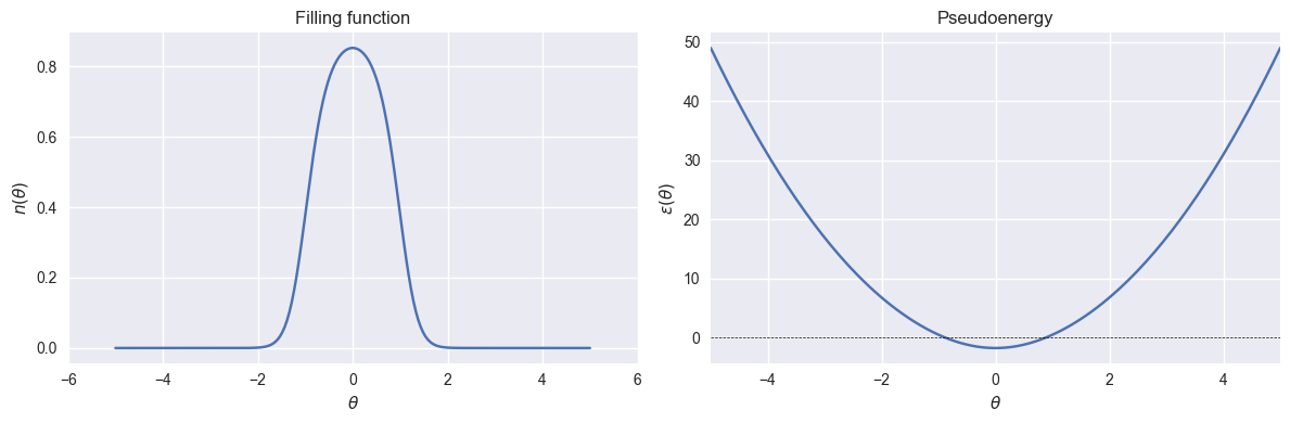
We solve the Yang-Yang equation at temperature \(T = 0.5\) and chemical potential \(\mu = 0.5\). The chemical potentials are passed as a dictionary keyed by charge order — charge 2 is the energy (\(\theta^2\)) and charge 0 is the particle number.

The inverse temperature \(\beta = 1/T\) multiplies the energy charge, and \(-\mu/T\) multiplies the particle number charge, giving the standard grand canonical driving term:

\[\epsilon_0(\theta) = \frac{\theta^2}{T} - \frac{\mu}{T}\]

T = 0.5
mu = 0.5

state = TBAState.from_betas(model, grid, betas={2: 1/T, 0: -mu/T})

# plot filling function
fig, axes = plt.subplots(1, 2, figsize=(12, 4))

#plot(state.filling, ax=axes[0])
axes[0].plot(grid.points, state.filling.values)
axes[0].set_xlabel(r'$\theta$')
axes[0].set_ylabel(r'$n(\theta)$')
axes[0].set_title('Filling function')
axes[0].set_xlim(-6, 6)

# plot pseudoenergy
epsilon = np.log((1 - state.filling.values) / state.filling.values)
axes[1].plot(grid.points, epsilon)
axes[1].set_xlabel(r'$\theta$')
axes[1].set_ylabel(r'$\epsilon(\theta)$')
axes[1].set_title('Pseudoenergy')
axes[1].set_xlim(-5, 5)
axes[1].axhline(0, color='k', linestyle='--', linewidth=0.5)

plt.tight_layout()
plt.show()

Thermodynamic quantities

From the filling function we can compute the particle density \(\rho_p(\theta)\), the state density \(\rho_s(\theta)\), and the effective velocity \(v^{eff}(\theta)\).

rho_p = state.rho_p()
rho_s = state.rho_s()
v_eff = state.v_eff()

fig, axes = plt.subplots(1, 3, figsize=(15, 4))

axes[0].plot(grid.points, rho_p.values)
axes[0].set_xlabel(r'$\theta$')
axes[0].set_ylabel(r'$\rho_p(\theta)$')
axes[0].set_title('Particle density')
axes[0].set_xlim(-6, 6)

axes[1].plot(grid.points, rho_s.values)
axes[1].set_xlabel(r'$\theta$')
axes[1].set_ylabel(r'$\rho_s(\theta)$')
axes[1].set_title('State density')
axes[1].set_xlim(-6, 6)

axes[2].plot(grid.points, v_eff.values)
axes[2].set_xlabel(r'$\theta$')
axes[2].set_ylabel(r'$v^{eff}(\theta)$')
axes[2].set_title('Effective velocity')
axes[2].set_xlim(-6, 6)

plt.tight_layout()
plt.show()

# total density
N_L = rho_p.integrate().values
print(f"Total particle density N/L = {N_L:.6f}")
print(f"Free energy density f = {state.free_energy():.6f}")

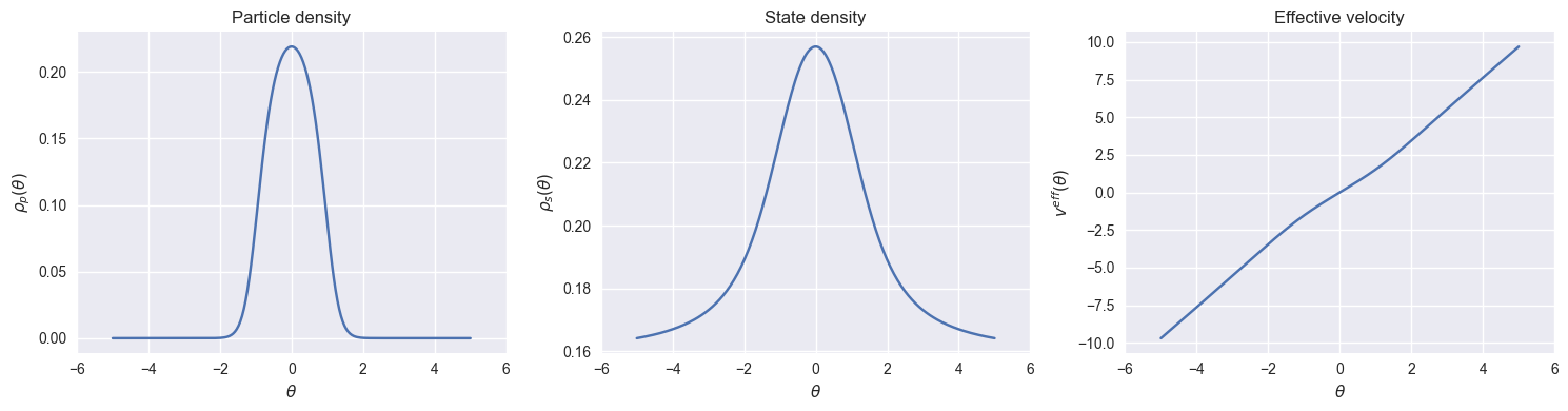
Total particle density N/L = 0.394173
Free energy density f = -0.464790

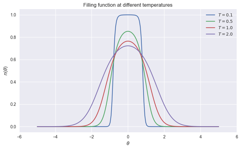
Temperature dependence

We now vary the temperature at fixed chemical potential and observe how the filling function evolves from the Fermi-Dirac distribution at high temperature to a step function at zero temperature.

temperatures = [0.1, 0.5, 1.0, 2.0]
mu = 0.5

fig, ax = plt.subplots(figsize=(8, 5))

for T in temperatures:
    state = TBAState.from_betas(model, grid, betas={2: 1/T, 0: -mu/T})
    ax.plot(grid.points, state.filling.values, label=f'$T={T}$')

ax.set_xlabel(r'$\theta$')
ax.set_ylabel(r'$n(\theta)$')
ax.set_title('Filling function at different temperatures')
ax.set_xlim(-6, 6)
ax.legend()
plt.tight_layout()
plt.show()

Zero temperature limit

At zero temperature all states below the Fermi rapidity \(\theta_F\) are filled. We construct the zero temperature state directly using TBAState.zero_temperature, which uses a Gauss-Legendre grid on \([-\theta_F, \theta_F]\).

theta_f = 2.0
state_T0 = TBAState.zero_temperature(model, theta_f=theta_f)

fig, axes = plt.subplots(1, 2, figsize=(12, 4))

axes[0].plot(state_T0.grid.points, state_T0.rho_p().values)
axes[0].set_xlabel(r'$\theta$')
axes[0].set_ylabel(r'$\rho_p(\theta)$')
axes[0].set_title(r'Particle density at $T=0$')

axes[1].plot(state_T0.grid.points, state_T0.v_eff().values)
axes[1].set_xlabel(r'$\theta$')
axes[1].set_ylabel(r'$v^{eff}(\theta)$')
axes[1].set_title(r'Effective velocity at $T=0$')

plt.tight_layout()
plt.show()

N_L = state_T0.rho_p().integrate().values
print(f"Total density N/L = {N_L:.6f}")
print(f"Fermi rapidity theta_F = {theta_f}")

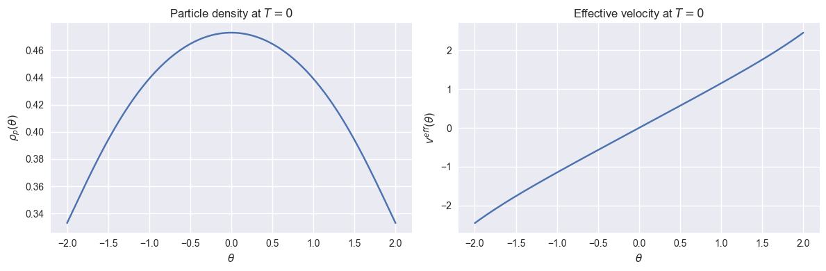
Total density N/L = 1.705870
Fermi rapidity theta_F = 2.0

Working at fixed density

In practice it is often more natural to specify the particle density \(N/L\) rather than the chemical potential. We use find_mu to find the chemical potential that reproduces the target density.

from rapidity.thermodynamics import find_mu

target_density = 1.0
T = 0.5

mu = find_mu(model, grid, density=target_density, T=T)
state = TBAState.from_betas(model, grid, betas={2: 1/T, 0: -mu/T})

print(f"Target density: {target_density}")
print(f"Chemical potential: mu = {mu:.6f}")
print(f"Achieved density: {state.rho_p().integrate().values:.6f}")

Target density: 1.0
Chemical potential: mu = 1.472007
Achieved density: 1.000000

References

• [YangYang1969] Yang, C. N., & Yang, C. P. (1969). Thermodynamics of a one-dimensional system of bosons with repulsive delta-function interaction. Journal of Mathematical Physics, 10(7), 1115-1122.

• [Takahashi1999] Takahashi, M. (1999). Thermodynamics of One-Dimensional Solvable Models. Cambridge University Press.